Dynamics

S-matrix and unitarity

Consider the process \(\ket{p_1 p_2, a}_\text{in} \rightarrow \ket{q_1 q_2, b}_\text{out}\). We define the scattering matrix \(\mathcal{S}\) which maps the in-states to out-states. The matrix elements will be given by

\[_{\text{out}}\!\bra{q_1 q_2,b} \mathcal{S} \ket{p_1 p_2,a}_\text{in} = (2\pi)^4\delta^4(p_1+p_2-q_1-q_2)\,\mathcal{S}_{ba}(q_1, q_2, p_1, p_2) \, .\]

We define the reaction amplitude \(\mathcal{M}\) using

\[_{\text{out}}\!\bra{q_1 q_2,b} \mathcal{S} - 1 \ket{p_1 p_2,a}_\text{in} = i(2\pi)^4\delta^4(p_1+p_2-q_1-q_2)\,\mathcal{M}_{ba}(q_1, q_2, p_1, p_2) \, .\]

Given

(21)\[\braket{q_1 q_2, b | p_1 p_2, a} = (2\pi)^4 \delta^{(4)} (p_1 - q_1) (2\pi)^4 \delta^{(4)} (p_2 - q_2) \, \delta_{ba} \, ,\]

we have

\[\mathcal{S}_{ba} (p_1, p_2, q_1, q_2) = (2\pi)^4 \delta^{(4)} (p_1 - q_1) \, \delta_{ba} + i \mathcal{M}_{ba}(q_1, q_2, p_1, p_2) \, .\]

We require \(\mathcal{S}\) to be unitary, i.e. \(\mathcal{S}^\dagger \mathcal{S} = \mathcal{S} \mathcal{S}^\dagger = 1\). Written in terms of the matrix elements,

\[\begin{split}&\braket{q_1 q_2, b | p_1 p_2, a} = \bra{q_1 q_2,b} \mathcal{S}^\dagger \mathcal{S} \ket{p_1 p_2,a} \\ &= \sum_c \int \frac{\text{d}^3 l_1}{(2\pi)^3 \, 2E_1} \frac{\text{d}^3 l_2}{(2\pi)^3 \, 2E_2} \bra{q_1 q_2,b} \mathcal{S}^\dagger \ket{l_1 l_2, c} \bra{l_1 l_2, c} \mathcal{S} \ket{p_1 p_2,a} \\ &= (2\pi)^4 \delta^{(4)}(p_1 + p_2 - q_1 - q_2) (2\pi)^4 \sum_c \int \text{d} \Phi_2 \, \mathcal{S}^*_{cb}(l_1, l_2, q_1, q_2) \mathcal{S}_{ca}(l_1, l_2, p_1, p_2) \, ,\end{split}\]

with \(\text{d}\Phi_2\) being the two-particle phase space measure, as defined in Eq. (19). Using Eq. (21) and factoring out one of the \(\delta\) functions, we get

\[(2\pi)^4 (p_1 - q_1) \, \delta_{ba} = (2\pi)^4 \sum_c \int \text{d} \Phi_2 \, \mathcal{S}^*_{cb}(l_1, l_2, q_1, q_2) \mathcal{S}_{ca}(l_1, l_2, p_1, p_2) \, .\]

Expressing this in terms of the \(\mathcal{M}\) matrix elements,

\[\begin{split}&\mathcal{M}_{ba}(p_1, p_2, q_1, q_2) - \mathcal{M}_{ab}^*(q_1, q_2, p_1, p_2) \\ &= i (2\pi)^4 \sum_c \int \text{d} \Phi_2 \, \mathcal{M}_{cb}^*(l_1, l_2, q_1, q_2) \mathcal{M}_{ca}(l_1, l_2, p_1, p_2) \, .\end{split}\]

Since \(\mathcal{M}_{ab}\) must be invariant under Lorentz transformations, one can (by slight abuse of notation) rewrite the above relation in terms of the Mandelstam variable \(s\) and the scattering angles,

\[\mathcal{M}_{ba}(s,\cos\theta) - \mathcal{M}_{ab}^*(s,\cos\theta) = i (2\pi)^4 \sum_c \int \text{d} \Phi_2 \, \mathcal{M}_{cb}^*(s,\cos\theta_q) \mathcal{M}_{ca}(s,\cos\theta_p) \, ,\]

where

\[\theta = \angle (\vec{p}_1, \vec{q}_1), \quad \theta_q = \angle (\vec{l}_1, \vec{q}_1), \quad \theta_p = \angle (\vec{l}_1, \vec{p}_1).\]

Using Eq. (20), we obtain the discontinuity relation for \(\mathcal{M}\),

(22)\[\begin{split}&\mathrm{Disc}(\mathcal{M}_{ba}(s,\cos\theta)) \equiv \mathcal{M}_{ba}(s,\cos\theta) - \mathcal{M}_{ab}^*(s,\cos\theta) \\ &= i \sum_c \rho_c(s) \int_{0}^{2\pi} \frac{\text{d}\phi_l}{2\pi} \int_{-1}^{+1} \text{d} \cos\theta_q \, \mathcal{M}_{cb}^*(s,\cos\theta_q) \mathcal{M}_{ca}(s,\cos\theta_p) \, .\end{split}\]

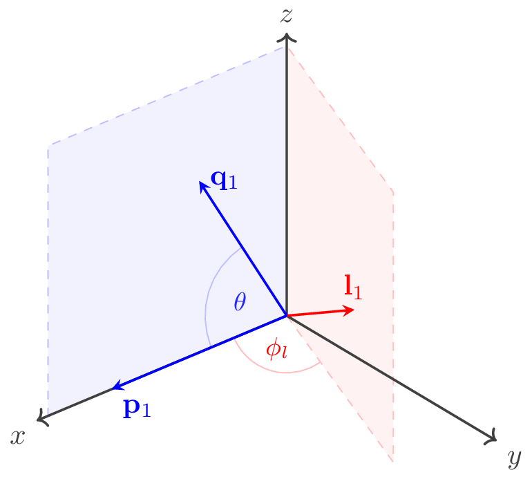
Note, that while the amplitudes \(\mathcal{M}_{ca/cb}\) do not explicitly depend on the azimuthal angles, the cosines of \(\theta_q\) and \(\theta_p\) depend on the azimuthal angle \(\phi_l\) of \(\vec{l}_1\) (see Fig. 6),

(23)\[\begin{split}\cos(\theta_q) = \cos(\theta)\cos(\theta_q) + \sin(\theta)\sin(\theta_q) \cos(\phi_l) \, , \\ \cos(\theta_p) = \cos(\theta)\cos(\theta_p) + \sin(\theta)\sin(\theta_p) \cos(\phi_l) \, .\end{split}\]

Fig. 6 Spatial configuration of \(\vec{p}_1\), \(\vec{q}_1\), and \(\vec{l}_1\). One can always rotate the coordinate system so that \(\vec{p}_1\) and \(\vec{q}_1\) fall onto e.g. the \(xz\)-plane. However, with a third momentum \(\vec{l}_1\), the case is necessarily 3-dimensional and we need to consider the azimuthal angle \(\phi_l\) (see Eq. (23) and the surrounding text for more details).

Partial wave expansion

Physical amplitudes are often decomposed in states of definite angular momentum. This is done by the so-called partial wave expansion,

(24)\[\mathcal{M}(s, \cos\theta) = \sum_{\ell=0}^{\infty} (2\ell+1) M_\ell(s) P_\ell(\cos\theta) \, ,\]

where \(M_\ell\) are called the partial waves and \(P_\ell\) denote the Legendre polynomials, given by

\[P_\ell(x) = \frac{1}{2^\ell \ell!} \frac{\text{d}^\ell}{\text{d} x^\ell} (x^2 - 1)^\ell \, .\]

They satisfy the orthogonality relations

\[\begin{split}&\int_{-1}^{+1} \text{d} x P_\ell(x) P_{\ell'}(x) = \frac{2}{2\ell+1} \delta_{\ell \ell'} \, , \\ &\sum_{\ell=0}^{\infty} P_\ell(x) P_\ell(y) = \frac{2}{2\ell+1} \delta(x - y) \, .\end{split}\]

With this, one can invert Eq. (24) to project the full amplitude on a specific partial wave,

(25)\[M_\ell(s) = \frac{1}{2} \int_{-1}^{+1} \text{d} \cos\theta \, \mathcal{M}(s, \cos\theta) P_\ell(\cos\theta) \, .\]

In order to plug this into Eq. (22), we first note, that [1]

(26)\[P_\ell(\cos\theta_q) = P_\ell(\cos\theta_q)P_\ell(\cos\theta) + 2 \sum_{k=1}^{\ell} \frac{(n-m)!}{(n+m)!} P_\ell^k(\cos\theta_q)P_\ell^k(\cos\theta) \cos(k \phi_l) \, ,\]

where \(P_\ell^k\) are the associated Legendre polynomials. The second summand in Eq. (26) vanishes after integrating over \(\phi_l\) and we obtain the discontinuity relation for the partial wave \(M_\ell\),

(27)\[\mathrm{Disc}(M_{ba,\ell}(s)) \equiv M_{ba,\ell}(s) - M_{ab,\ell}^*(s) = 2i \sum_c \rho_c(s) M_{cb,\ell}^*(s) M_{ca,\ell}(s) \, .\]