Complex analysis

Complex field

Consider the group \(\mathbb{R}^2 \equiv \mathbb{R} \times \mathbb{R}\) which is a set of 2-dimensional vectors, closed under a binary operation we call “addition” (\(+\)),

(1)\[\begin{split}\mathrm{add} : \mathbb{R}^2 \times \mathbb{R}^2 &\rightarrow \mathbb{R}^2 , \\ ((a_1, a_2), (b_1, b_2)) &\mapsto (a_1, a_2) + (b_1, b_2) = (a_1 + b_1, a_2 + b_2) \, .\end{split}\]

One can define another binary operator called “multiplication”,

(2)\[\begin{split}\mathrm{mult} : \mathbb{R}^2 \times \mathbb{R}^2 &\rightarrow \mathbb{R}^2 , \\ ((a_1, a_2), (b_1, b_2)) &\mapsto (a_1, a_2)(b_1, b_2) = (a_1 b_1 - a_2 b_2, a_1 b_2 + a_2 b_1) \, .\end{split}\]

We can check that these two binary operations satisfy the field axioms. We call the resulting field the complex field \(\mathbb{C}\). It is common to denote the basis elements by

\[(1, 0) \equiv 1, \qquad (0, 1) \equiv i,\]

where the corresponding components are called the “real” and “imaginary” parts of a complex number. With this, one can write for \(z\in\mathbb{C}\),

\[z = \mathrm{Re}(z) + i \, \mathrm{Im}(z).\]

The multiplication operator defined via Eq. (2) has two important features:

1. The subfield \(\{z \in \mathbb{C} \,|\, z = (z_1, 0)\}\) forms the real field \(\mathbb{R}\) under the usual multiplication of numbers.

2. \(i^2 = -1\), which provides a solution to a polynomial equation, \(x^2 + 1 = 0\).

This hints at the fact that the complex field \(\mathbb{C}\) is an algebraic closure of \(\mathbb{R}\) [A field \(F\) is algebraically closed if every non-constant polynomial with coefficients in \(F\) also has a solution in \(F\). The polynomial \(x^2+1\) can be used as a counter-example to show that \(\mathbb{R}\) is not algebraically closed. One can prove, on the other hand, that \(\mathbb{C}\) is (see e.g. ).]. The additional dimension along \(i = (0,1)\) is called the “imaginary axis” due to historic reasons. An important unary operation called “complex conjugation” (\({}^*\)) is defined to invert the imaginary component of a complex number,

(3)\[\begin{split}\mathrm{conj} : \mathbb{C} &\rightarrow \mathbb{C} , \\ (z_1, z_2) &\mapsto (z_1, z_2)^* = (z_1, -z_2) \, .\end{split}\]

Complex numbers are commonly represented using polar coordinates \(r\in[0,\infty)\) and \(\theta\in[0,2\pi)\),

(4)\[z = r e^{i\theta} = r \cos(\theta) + i \, r \sin(\theta) \, .\]

One can check, that

\[\begin{split}r^2 &= \left(\mathrm{Re}(z)\right)^2 + \left(\mathrm{Im}(z)\right)^2 = z z^* \equiv |z|^2 \, , \\ \theta &= \tan^{-1}(\mathrm{Im}(z) / \mathrm{Re}(z)) \equiv \mathrm{arg}(z) \, .\end{split}\]

Functions and analyticity

Consider a function \(f(z)\) defined on a domain \(z \in \mathcal{D}\). We call this function differentiable at a point \(z_0\) if the limit

\[\lim_{z \to z_0} \frac{f(z) - f(z_0)}{z - z_0} \equiv f'(z_0)\]

exists. If \(f\) is differentiable at each point of \(\mathcal{D}\), we call it analytic in \(\mathcal{D}\). The limit should exist irrespective of how \(z\) approaches \(z_0\), which leads to the Cauchy–Riemann conditions: if \(f \equiv u + i v\) is analytic in \(\mathcal{D}\), then throughout \(\mathcal{D}\) it satisfies [The proof is very simple and can be found in many textbooks on complex analysis, e.g. [6].]

\[\frac{\partial u}{\partial x} = \frac{\partial v}{\partial y}, \quad \frac{\partial u}{\partial y} = -\frac{\partial v}{\partial x}.\]

Poles and the residue theorem

A very important result for analytic functions is the Cauchy’s theorem, which states that for an analytic function \(f\) in \(\mathcal{D}\) and a piecewise smooth closed curve \(\mathcal{C}\) in \(\mathcal{D}\) we have

(5)\[\oint_{\mathcal{C}} f(z) \text{d} z = 0 \, .\]

If \(f\) contains isolated singularities \(\{z_1, z_2, \dots, z_n\}\), the residue theorem states

(6)\[\oint_{\mathcal{C}} f(z) \text{d} z = 2\pi i \sum_{z_k \text{ inside } \mathcal{C}} \mathrm{Res}(f; z_k) \, ,\]

where \(\mathrm{Res}(f; z_k)\) is called the residue of \(f\) at point \(z_k\) and can be computed for simple poles via

(7)\[\mathrm{Res}(f; z_k) = \lim_{z \to z_k} (z - z_k) f(z) \, .\]

This leads to the Cauchy’s integral formula. Suppose \(f\) is analytic in \(\mathcal{D}\). Then, for a piecewise smooth, positively oriented simple closed curve \(\mathcal{C}\) whose inside \(\mathcal{D}_{\mathcal{C}}\) also lies in \(\mathcal{D}\), one has

(8)\[f(z) = \frac{1}{2\pi i} \oint_{\mathcal{C}} \frac{f(w) \text{d} w}{w-z} \, , \qquad \text{for all } z \in \mathcal{D}_{\mathcal{C}}.\]

This formula will be exploited heavily in the section about dispersion relations.

Roots, logarithms, and branch cuts

The square root of a number \(x\) is introduced to solve the equation of type

\[y^2 = x.\]

Due to the surjective nature of the square, there is a sign ambiguity in defining the square root,

\[\sqrt{x}^{I} = y, \quad \text{or} \quad \sqrt{x}^{II} = -y,\]

where we conventionally choose \(\sqrt{x}\equiv\sqrt{x}^{I}\). This ambiguity has a special importance in the context of complex numbers and is connected with a concept called Riemann sheets. To see this connection, consider taking a square root of Eq. (4),

\[\sqrt{z} = \sqrt{r e^{i\theta}} = \sqrt{r} e^{i\theta/2} .\]

This makes it clear that \(\sqrt{z}\) has no limit at \(\theta=0\),

\[\lim_{\theta \rightarrow 0^+} \sqrt{r e^{i\theta}} = \sqrt{r} \neq \sqrt{r} e^{i\pi} = \lim_{\theta \rightarrow 2\pi^-} \sqrt{r e^{i\theta}} \, .\]

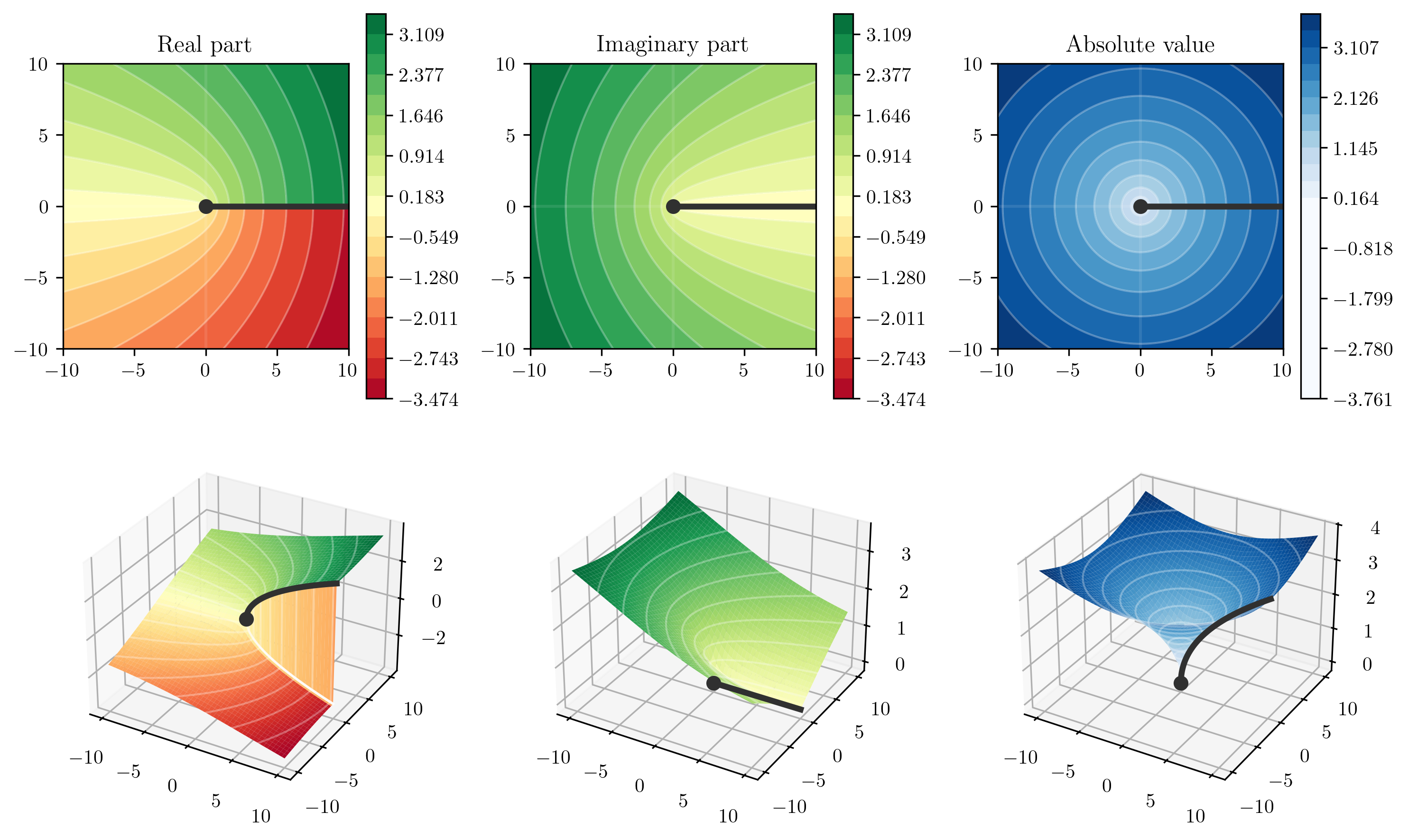
Fig. 1 Complex plot of \(\sqrt{z}\) on the first Riemann sheet.

In complex analysis this type of discontinuity is referred to as a branch cut and is illustrated on Fig. 1. Noting that \(e^{i\pi} = -1\), one can recognize

\[\begin{split}\lim_{\theta \rightarrow 0^+} \sqrt{r e^{i\theta}} &= \sqrt{r}^{I} , \\ \lim_{\theta \rightarrow 2\pi^-} \sqrt{r e^{i\theta}} &= \sqrt{r}^{II} .\end{split}\]

For a general case, one defines

\[\begin{split}\sqrt{z}^{I} &= \sqrt{|z|} e^{i \arg{z}/2} , \\ \sqrt{z}^{II} &= \sqrt{|z|} e^{i (\arg{z}+2\pi)/2} = |z| e^{i \arg{z}/2} e^{i\pi}.\end{split}\]

The superscripts \(I,II\) enumerate the Riemann sheets for the square root. Note, that since \(e^{i (\arg{z}+4\pi)/2} = e^{i \arg{z}/2} e^{i2\pi} = e^{i \arg{z}/2}\), square root has only two sheets, which are smoothly connected along the branch cut. Correspondingly, \(n^{\text{th}}\) roots have \(n\) Riemann sheets,

\[\begin{split}\sqrt[n]{z}^{I} &= \sqrt[n]{|z|} e^{i \arg{z}/n} , \\ \sqrt[n]{z}^{II} &= \sqrt[n]{|z|} e^{i (\arg{z}+2\pi)/n} , \\ \sqrt[n]{z}^{III} &= \sqrt[n]{|z|} e^{i (\arg{z}+4\pi)/n} , \\ &\vdots\end{split}\]

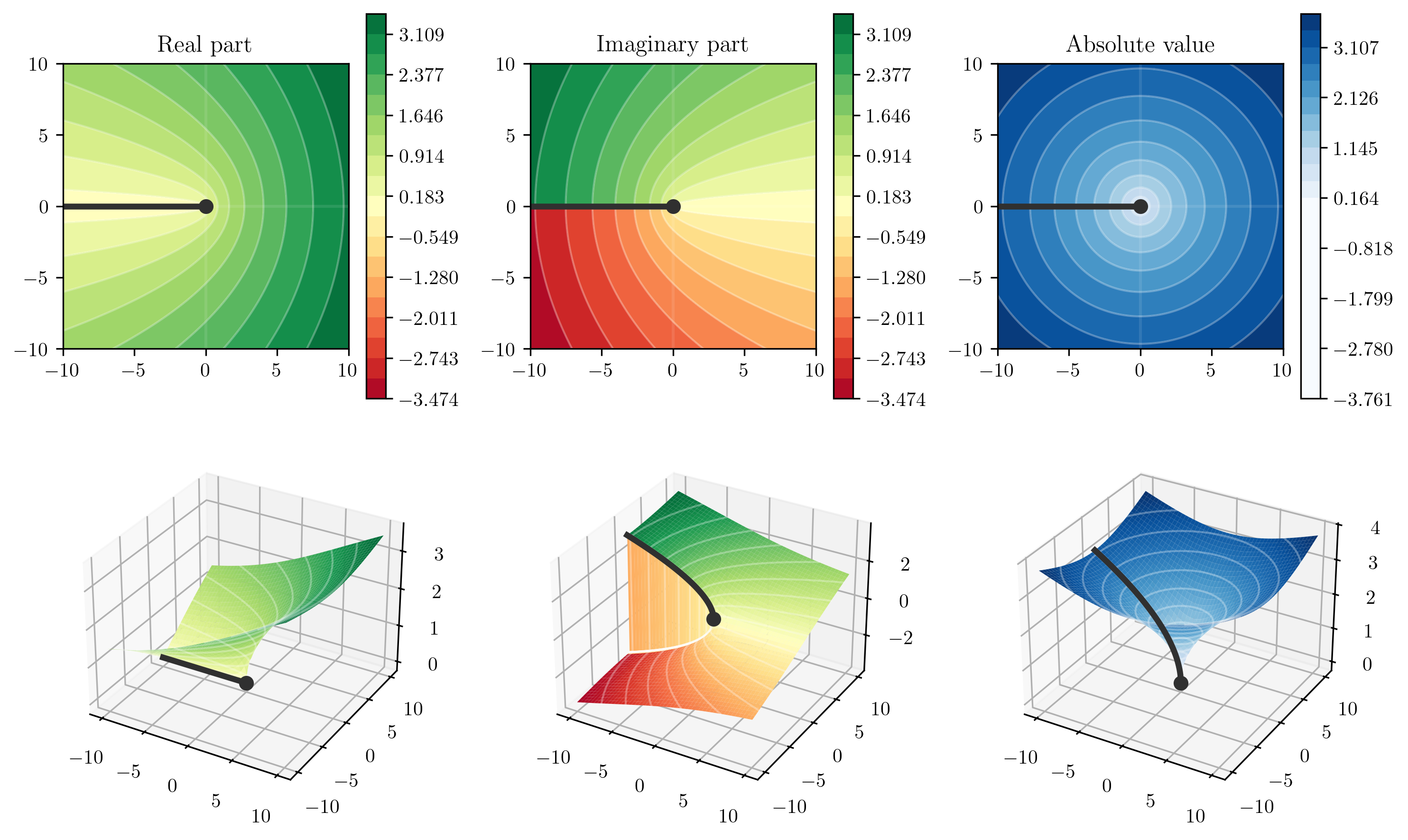
Fig. 2 Complex plot of \(\sqrt{z}\) on the first Riemann sheet, with a left-hand cut according to numpy conventions [8]. Note, that in contrast with the plots on Fig. 1, here the cut is placed in the imaginary part.

Another relevant example of a function with a branch cut is the logarithm,

\[\log(z) = \log(r e^{i\theta}) = \log(r) + i\theta .\]

Since \(\log\) turns \(\theta\) into imaginary part, it loses the cyclic property and we end up with infinite amount of Riemann sheets,

\[\begin{split}\log^{I}(z) &= \log(r) + i\theta , \\ \log^{II}(z) &= \log(r) + i\theta + i2\pi , \\ \log^{III}(z) &= \log(r) + i\theta + i4\pi , \\ &\vdots\end{split}\]

Finally, we note that the position of the branch cut depends on the convention. Many numeric packages define \(\theta \in (-\pi, \pi]\), which sets the branch cut on the left side of the complex plane, as depicted on Fig. 2. Throughout this thesis, we refer to the special cases of branch cuts at \(\theta=0\) and \(\theta=\pi\) as right-hand cut (RHC) and left-hand cut (LHC), correspondingly.