Dispersion relations

Kramers–Kronig relations

In this section we take a closer look at Eq. (8). Since the Cauchy’s integral formula assumes analyticity inside the integration curve, we need to choose the curve \(\mathcal{C}\) in such a way that it

1. encloses the Cauchy pole,

2. excludes the non-analytic parts of \(f\).

For simplicity, consider a complex function \(f(z)\) that is analytic on the entire \(\mathbb{C}\) except for a single branch cut, spanning a subset of the real line. Then, \(\mathbb{C}\) can be deformed as depicted in Fig. 3. This results into three contributions to Eq. (8), namely,

(9)\[f(s) = \frac{\lim_{\epsilon \to 0}}{2\pi i} \bigg( \underbrace{\int_{s_{\text{thr}}}^{R} \frac{f(z + i\epsilon) \text{d} z}{z-s}}_{\text{above the branch cut}} + \underbrace{\int_{R}^{s_{\text{thr}}} \frac{f(z - i\epsilon) \text{d} z}{z-s}}_{\text{below the branch cut}} + \underbrace{i \int_{0}^{2\pi} \frac{f(R e^{i\theta}) R e^{i\theta} \text{d} \theta}{R e^{i\theta}-s}}_{\text{arc}} \bigg) ,\]

where \(s_{\text{thr}}\) is the beginning of the branch cut (i.e. a “threshold”) and \(R\) is the radius of the arc. If \(f(R e^{i\theta})\) drops for large values of \(R\) (which is typically the case for physical amplitudes), the arc contribution can be neglected and in the limit of \(R \to \infty\) we have

(10)\[\begin{split}f(s) &= \frac{1}{2\pi i} \lim_{\epsilon \to 0} \bigg( \int_{s_{\text{thr}}}^{\infty} \frac{f(z + i\epsilon) \text{d} z}{z-s} + \int_{\infty}^{s_{\text{thr}}} \frac{f(z - i\epsilon) \text{d} z}{z-s} \bigg) \\ &= \frac{1}{2\pi i} \lim_{\epsilon \to 0} \int_{s_{\text{thr}}}^{\infty} \frac{\left(f(z + i\epsilon) - f(z - i\epsilon)\right) \text{d} z}{z-s} \, .\end{split}\]

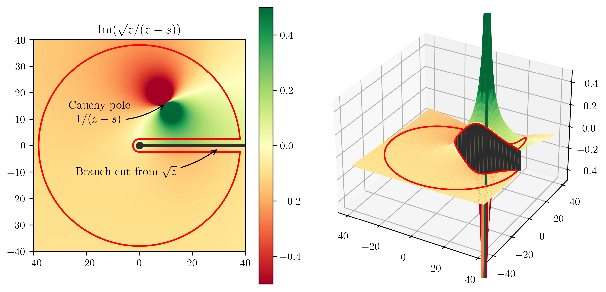
Fig. 3 Integration contour (red curve) for the Cauchy’s integral formula for \(f(z)=\sqrt{z}\).

The term in brackets \(\left(f(z + i\epsilon) - f(z - i\epsilon)\right)\) is often denoted as \(\mathrm{Disc}(f(z))\). If a function \(f\) is real on a finite segment of the real axis, the Schwarz reflection principle states that for a domain \(\mathcal{D}\) enclosing this finite segment, if \(f\) is analytic in \(\mathcal{D}\),

\[f(z^*) = (f(z))^* \quad \text{for } z \in \mathcal{D} \, .\]

If this condition holds, we can rewrite

\[\mathrm{Disc}(f(z)) = \left(f(z + i\epsilon) - f(z + i\epsilon)^*\right) = 2i \, \mathrm{Im}(f(z)) \,\]

and therefore,

(11)\[f(s) = \frac{1}{\pi} \int_{s_{\text{thr}}}^{\infty} \frac{\mathrm{Im}(f(z)) \text{d} z}{z-s} \, .\]

If we take out the Cauchy pole contribution using the Sokhotski–Plemelj theorem ,

(12)\[\lim_{\epsilon \to 0^+} \frac{1}{x \pm i\epsilon} = \mp i\pi\delta(x) + \mathcal{P}\!\left(\frac{1}{x}\right) \, ,\]

we arrive at

(13)\[\mathrm{Re}(f(s)) = \frac{1}{\pi} \mathcal{P}\!\!\int_{s_{\text{thr}}}^{\infty} \frac{\mathrm{Im}(f(z)) \text{d} z}{z-s} \, ,\]

where \(\mathcal{P}\!\!\int\) denotes the Cauchy principal value integral. Both Eq. (11) and Eq. (13) are forms of the Kramers–Kronig relations and demonstrate how a function \(f\) can be reconstructed on \(z\in\mathcal{D}\) using the knowledge of just the non-analytic parts as an input. If \(f\) has poles in addition to the branch cut(s), one needs to add the corresponding residues to these relations.

Subtractions

Eq. (11) is often referred to as an unsubtracted dispersion relation and has a clear caveat: the convergence behaviour depends on the asymptotics of the branch cut. If \(\mathrm{Im}(f(z))\) grows fast enough as \(z \to \infty\), the integral diverges. To cure this, we may exploit the fact that \(f\) is analytic at \(f(s_0 < s_\text{thr})\). Define

(14)\[g(s) = \frac{f(s) - f(s_0)}{s - s_0} \, .\]

Since \(f\) is analytic at \(s_0\), \(g\) is regular there and, at the same time, drops faster than \(f\) by one power in \(s\). Therefore, one can write an unsubtracted dispersion relation

\[g(s) = \frac{1}{\pi} \int_{s_{\text{thr}}}^{\infty} \frac{\mathrm{Im}(g(z)) \text{d} z}{z-s}\]

and using Eq. (14) arrive at

\[f(s) = f(s_0) + \frac{s-s_0}{\pi} \int_{s_{\text{thr}}}^{\infty} \frac{\mathrm{Im}(f(z)) \text{d} z}{(z-s_0)(z-s)} \, .\]

We can repeat this procedure \(n\) times to arrive at

(15)\[f(s) = \sum_{k=0}^{n-1} \underbrace{\frac{f^{(k)}(s_0)}{k!}}_{f_k} (s-s_0)^{k} + \frac{(s-s_0)^n}{\pi} \int_{s_{\text{thr}}}^{\infty} \frac{\mathrm{Im}(f(z)) \text{d} z}{(z-s_0)^n(z-s)} \, .\]

Eq. (15) is called the nth subtracted dispersion relation and in contrast with Eq. (11), needs \(n\) subtraction constants \(f_k\) as part of the input.

Integrating over the Cauchy kernel

Taking an integral with a Cauchy singularity can become numerically unstable. To solve this issue, one usually separates

(16)\[\begin{split}\int_{s_{\text{thr}}}^{\infty} \frac{\mathrm{Im}(f(z)) \text{d} z}{(s-s_0)^n(s-z)} &= \int_{s_{\text{thr}}}^{\infty} \frac{\left(\mathrm{Im}(f(z))-\mathrm{Im}(f(s))\right) \text{d} z}{(z-s_0)^n(s-z)} \\ &+ \mathrm{Im}(f(s)) \int_{s_{\text{thr}}}^{\infty} \frac{\mathrm{Im}(f(z)) \text{d} z}{(z-s_0)^n(z-s)} \, ,\end{split}\]

where the integral

\[\mathcal{I}_{-n}(s, s_0; s_\text{thr}, \infty) \equiv \int_{s_{\text{thr}}}^{\infty} \frac{\mathrm{Im}(f(z)) \text{d} z}{(z-s_0)^n(z-s)}\]

is independent of \(f\) and can be computed analytically,

\[\mathcal{I}_{-n}(s, s_0; s_{\text{\text{thr}}}, \infty) = (s-s_0)^{-n} \left( \log\left(\frac{z-s}{z-s_0}\right) + \sum_{k=1}^{n-1} \frac{1}{k} \frac{(s-s_0)^{k}}{(z-s_0)^{k}} \right)\bigg|_{z=s_{\text{\text{thr}}}}^{z=\infty} \, .\]

Given that \(\mathrm{Im}(f(z))\) (i.e. the discontinuity itself) is differentiable along the cut, the first term of Eq. (16) has a regular integrand at \(z=s\) and one can take the integral without numerical complications. It is instructive to take explicit look at this for a once-subtracted case,

(17)\[\begin{split}f(s) &= f(s_0) + \frac{s-s_0}{\pi} \int_{s_{\text{thr}}}^{\infty} \frac{\left(\mathrm{Im}(f(z))-\mathrm{Im}(f(s))\right) \text{d} z}{(z-s_0)(z-s)} + \frac{\mathrm{Im}(f(s))}{\pi} \log\left(\frac{s_{\text{thr}}-s_0}{s_{\text{thr}}-s}\right) \\ &= \underbrace{f(s_0) + \frac{s-s_0}{\pi} \int_{s_{\text{thr}}}^{\infty} \frac{\left(\mathrm{Im}(f(z))-\mathrm{Im}(f(s))\right) \text{d} z}{(z-s_0)(z-s)} + \frac{\mathrm{Im}(f(s))}{\pi} \log\left(\left|\frac{s_{\text{thr}}-s_0}{s_{\text{thr}}-s}\right|\right)}_{\text{real part}} \\ &+ i \, \underbrace{\mathrm{Im}(f(s)) \, \theta(s-s_\text{thr})}_{\text{imaginary part}} \, ,\end{split}\]

where we have used

\[\log(-r) = \log(r e^{i\pi}) = \log(r) + i\pi \, .\]

Eq. (17) shows how the dispersion integral reproduces the input \(\mathrm{Im}(f(s))\) by definition.