Utilities#

dispersionrelations.utils.sqrt_custom_branch_cut(z, t_bc, sheet=1)[source]#

Square root with a custom branch cut in the real part.

Parameters:

z (array_like) – A complex number or sequence of complex numbers.
t_bc (float) – The angle of the branch cut in radians.
sheet (int) – The sheet of the square root function. Must be 1 or 2.

Returns:

w – The same shape as input z.

Return type:

array_like

Raises:

ValueError – If sheet is not 1 or 2.

Examples

Complex plot of sqrt_custom_branch_cut(z, t_bc=np.pi/7):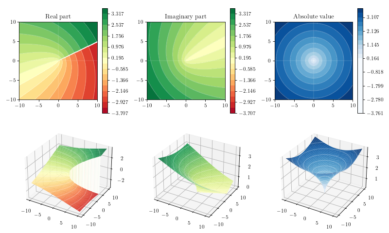

dispersionrelations.utils.sqrtRHC(z, sheet=1)[source]#

Square root with the right-hand-cut \(z\in[0,\infty)\) in the real part.

Parameters:

z (array_like) – A complex number or sequence of complex numbers.
sheet (int) – The sheet of the square root function. Must be 1 or 2.

Returns:

w – The same shape as input z.

Return type:

array_like

Raises:

ValueError – If sheet is not 1 or 2.

Examples

Complex plot of sqrtRHC: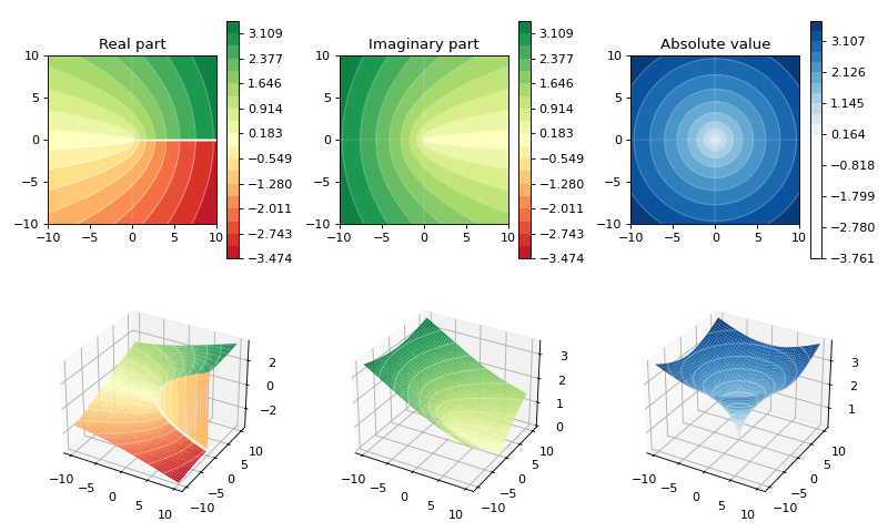

dispersionrelations.utils.sqrtLHC(z, sheet=1)[source]#

Square root with the left-hand-cut \(z\in(-\infty,0]\) in the real part.

Parameters:

z (array_like) – A complex number or sequence of complex numbers.
sheet (int) – The sheet of the square root function. Must be 1 or 2.

Returns:

w – The same shape as input z.

Return type:

array_like

Raises:

ValueError – If sheet is not 1 or 2.

Examples

Complex plot of sqrtLHC: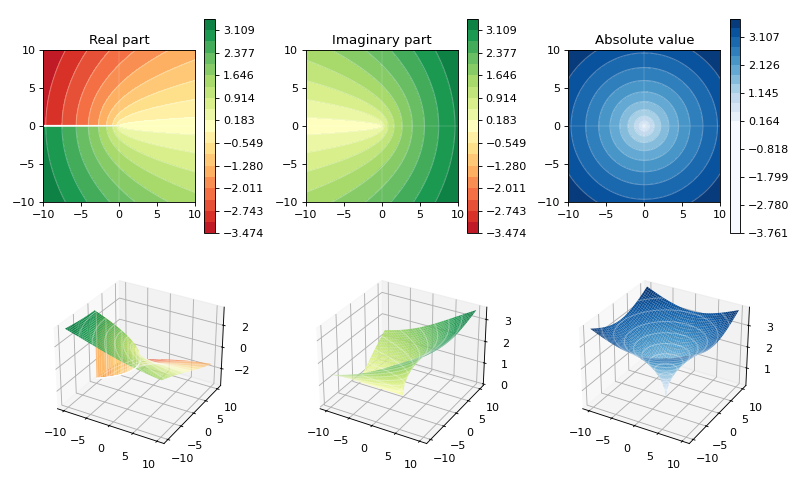

One can compare this to the numpy implementation np.sqrt, where the cut is in the imaginary part: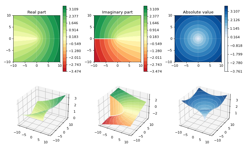

dispersionrelations.utils.log_custom_branch_cut(z, t_bc)[source]#

Logarithm with a custom branch cut.

Parameters:

z (array_like) – A complex number or sequence of complex numbers.
t_bc (float) – The angle of the branch cut in radians.

Returns:

w – The same shape as input z.

Return type:

array_like

Examples

Complex plot of log_custom_branch_cut(z, t_bc=-np.pi/2):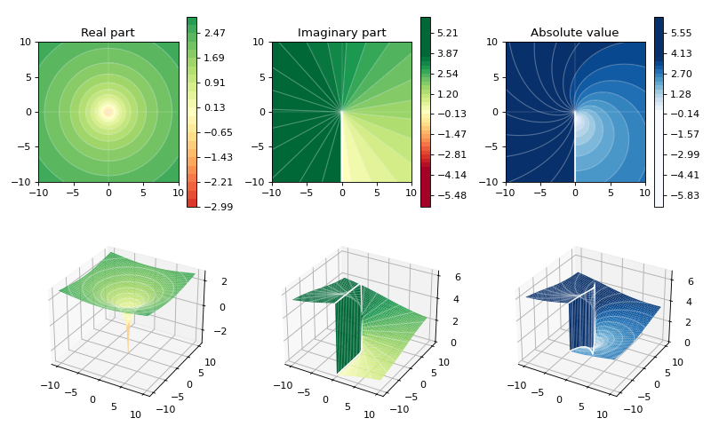

dispersionrelations.utils.logRHC(z)[source]#

Logarithm with the right-hand-cut \(z\in[0,\infty)\).

Parameters:: z (array_like) – A complex number or sequence of complex numbers.
Returns:: w – The same shape as input z.
Return type:: array_like

Examples

Complex plot of logRHC: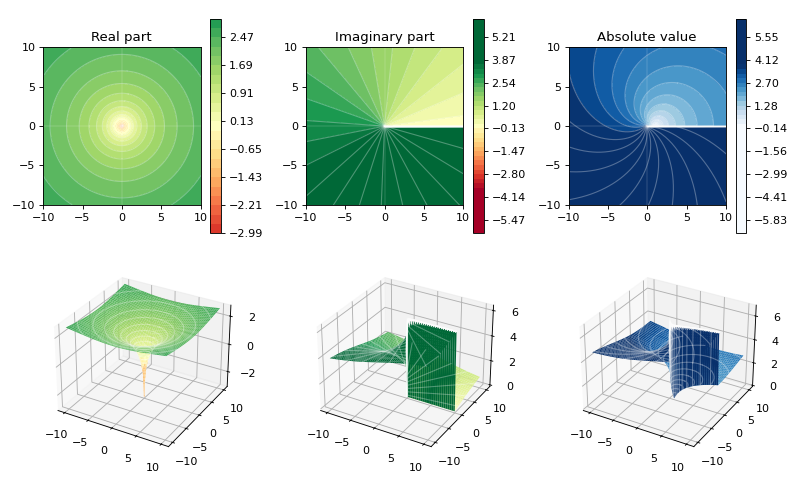

dispersionrelations.utils.logLHC(z)[source]#

Logarithm with the left-hand-cut \(z\in(-\infty,0]\).

Parameters:: z (array_like) – A complex number or sequence of complex numbers.
Returns:: w – The same shape as input z.
Return type:: array_like

Examples

Complex plot of logLHC: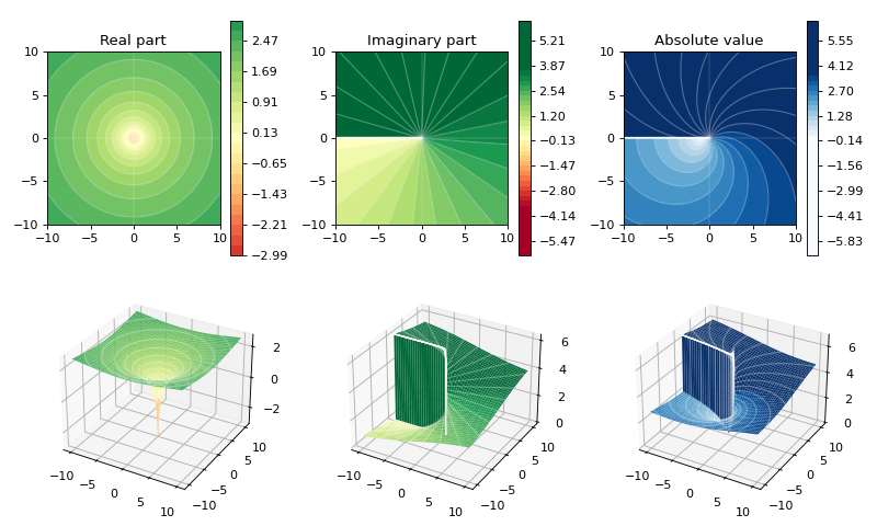

dispersionrelations.utils.logC(z)[source]#

Logarithm convention used for Cauchy integrals (right-hand-cut).

Parameters:: z (array_like) – A complex number or sequence of complex numbers.
Returns:: w – The same shape as input z.
Return type:: array_like

Examples

Complex plot of logC: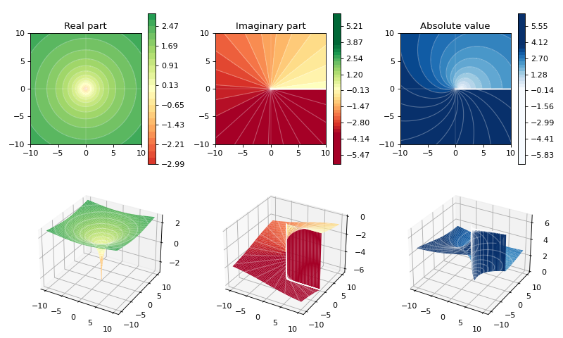

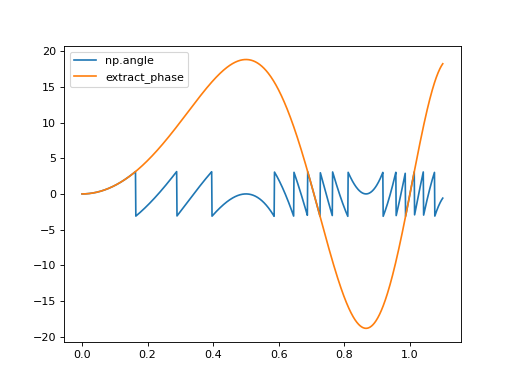
dispersionrelations.utils.extract_phase(f, jump=1.5)[source]#

Extraction of continuous phase (angle).

Parameters:

f (array_like) – A sequence of complex numbers.
jump (float) – The amount (in radians) by which the phase may jump along discontinuous points (depends on resolution).

Returns:

t – The same shape as input f.

Return type:

array_like

Examples

>>> import numpy as np
>>> import matplotlib.pyplot as plt
>>> from dispersionrelations.utils import extract_phase
>>> E_1 = np.linspace(0, 1.1, 1000)
>>> s_1 = E_1 ** 2
>>> f_1_r = np.exp(-(s_1)**2)
>>> f_1_θ = 2*np.pi * 3 * np.sin(2*np.pi * s_1)
>>> f_1 = f_1_r * np.exp(1j * f_1_θ)
>>> plt.plot(E_1, np.angle(f_1))
>>> plt.plot(E_1, extract_phase(f_1))

dispersionrelations.utils.conformal_variable(s, sE, sL)[source]#

Conformal variable, as defined in e.g. [9].

Parameters:

s (array_like) – A complex number or sequence of complex numbers.
sE (float) – Some conveniently chosen expansion point.
sL (float) – The location of the closest branch point of the LHC.

Returns:

ω – The same shape as input s.

Return type:

array_like

Notes

The conformal variable is defined as

\[\omega(s, s_E, s_L) = \frac{\sqrt{s - s_L} - \sqrt{s_E - s_L}}{\sqrt{s - s_L} + \sqrt{s_E - s_L}}.\]

dispersionrelations.utils.cite(ref)[source]#

Produces a LaTeX citation command.

Parameters:: ref (str) – The reference key.
Returns:: citation – The LaTeX citation command cite{ref}.
Return type:: str

See also

cite: Forward operation.

dispersionrelations.utils.save_to_json(data, filename: str = None, folder: str = '', metadata: dict = {})[source]#

Saves a dictionary to a JSON file.

Parameters:

data (dict) – The data to be saved.
filename (str) – The name of the file to save the data to. If None, the current date and time will be used.
folder (str) – The folder to save the file in. Default is the current folder.
metadata (dict) – Additional metadata to be included in the JSON file. Default is an empty dictionary.

Return type:

None

dispersionrelations.utils.load_from_json(filename: str, folder: str = '')[source]#

Loads a dictionary from a JSON file.

Parameters:

filename (str) – The name of the file to load the data from.
folder (str) – The folder to load the file from. Default is the current folder.

Returns:

data – The loaded data.

Return type:

dict

dispersionrelations.utils.scientific_notation(num, rounding=2)[source]#

Scientific notation.

Parameters:

num (float) – A real number.
rounding (int) – Number of digits after the period.

Returns:

num_not – A LaTeX code for the number representation.

Return type:

str

Examples

>>> import numpy as np
>>> from DispersionRelations.constants import scientific_notation
>>> print(scientific_notation(np.pi))
'3.1415926536'
>>> print(scientific_notation(13.4))
'1.34 \\times 10^{1}'

dispersionrelations.utils.rounding_PDG(mean, std)[source]#

Rounding with PDG rules [14].

Parameters:

mean (float) – Mean value of the quantity.
std (float) – Standard deviation of the quantity.

Returns:

mean_out, std_out – Mean value and standard deviation, cited according to the PDG prescription.

Return type:

(float, float)

Examples

>>> from DispersionRelations.constants import rounding_PDG
>>> print(rounding_PDG(0.827, 0.119))
(0.83, 0.12)
>>> print(rounding_PDG(0.827, 0.367))
(0.8, 0.4)